A Datalog relation is a set of ordered tuples. During evaluation, rules add tuples; after the relation’s final producer has run, later rules may only look up or scan its contents. This suggests using one representation while the relation grows and another after it becomes read-only. We benchmark six candidate strategies to understand the trade-offs behind that choice.
The work is motivated by the interpreter’s B-tree relation machinery, which is instantiated for a fixed set of compile-time arities. A dynamic-arity B-tree chooses its tuple width when it is constructed, avoiding a separate template instantiation for each width. This benchmark compares that prototype with static B-trees, ordered sets, and vector-based strategies. It measures the containers in isolation; it does not integrate the dynamic B-tree into relation evaluation or measure the cost of switching representations during evaluation.
The strategies
The benchmark compares six ways to hold the same tuples:
| Strategy | Tuple representation | How insertion/build works |
|---|---|---|
| Dynamic B-tree | Runtime-sized std::vector<RamDomain> keys |
Insert each tuple into the dynamic B-tree, ignoring duplicates. |
| Static B-tree | Fixed-size Tuple<RamDomain, Arity> keys |
Insert each tuple into the interpreter’s statically instantiated B-tree. |
Dynamic std::set |
Runtime-sized vectors | Insert into std::set with a runtime-arity lexicographic comparator. |
Static std::set |
Fixed-size tuple keys | Insert into std::set using the fixed tuple’s ordering. |
| Sorted vector | A vector of separately allocated dynamic tuples | Append all tuples, sort them, and erase adjacent duplicates. |
| Flat vector | One contiguous buffer of tuple columns | Store all tuple values contiguously, sort row indices, reorder the buffer in place, and compact duplicates. |
The static strategies are measured at arities 1 through 22. Dynamic strategies also run at arity 32. The results therefore reflect tuple representation and comparator costs as well as container behavior; they are not a container-only comparison.
The charts compress the unmeasured arities 23–31: arity 32 appears in a separate position after 22, with an axis-break mark and dashed guides between the dynamic strategies’ measured endpoints. The x-axis labels retain the actual arities.
What the experiment measures
Each workload makes 500,000 insertion attempts at three duplicate rates. That yields 500,000 distinct tuples at 0% duplicates, 250,000 at 50%, and 50,000 at 90%. For each rate, we use two tuple-distribution profiles with the same row IDs and shuffled attempt order:
- Early discriminator: the first column is a row ID, and remaining columns are deterministically derived from it. Distinct tuples differ immediately in the first column.
- Late discriminator: all columns before the last are zero, and the last column is the row ID. Distinct tuples share a prefix and differ only at the final column.
The profiles are identical at arity 1, where the only column is both first and last. All strategies receive identical tuples within a profile. These two workloads isolate how the position of the first differing column affects lexicographic comparisons.
For each strategy, the benchmark records three phases:
- Insert/build: insert all attempts into a tree or set, or construct and sort/deduplicate a vector representation.
- Lookup: look up all 500,000 attempted tuples. These are all exact-match hits.
- Scan: visit every distinct stored tuple and compute a checksum.
Each case is repeated five times, and the CSV reports the median timing in milliseconds. The distinct_tuples, hits, and checksum columns also let the benchmark check that each implementation produced the same result. The flat-vector path materializes its contiguous tuple buffer inside the timed build phase; the other strategies receive their generated input rows before that phase. The insertion numbers therefore include each strategy’s representation-specific build work.
Test machine and build
The reported run was collected on a machine with an Intel Core i7-14700K (20 cores, 28 hardware threads) and 64 GB of RAM. It ran Fedora Linux 44 with kernel 7.2.5. The benchmark was built in CMake Release mode with GCC 16.2.1 and no additional C++ compiler flags. Its tuples use 32-bit RamDomain values (RAM_DOMAIN_SIZE=32): the standalone benchmark target has no explicit domain-size definition, so it uses the default from RamTypes.h. This may differ from the main Soufflé libraries, which can be configured for 64-bit domains.
What the results say
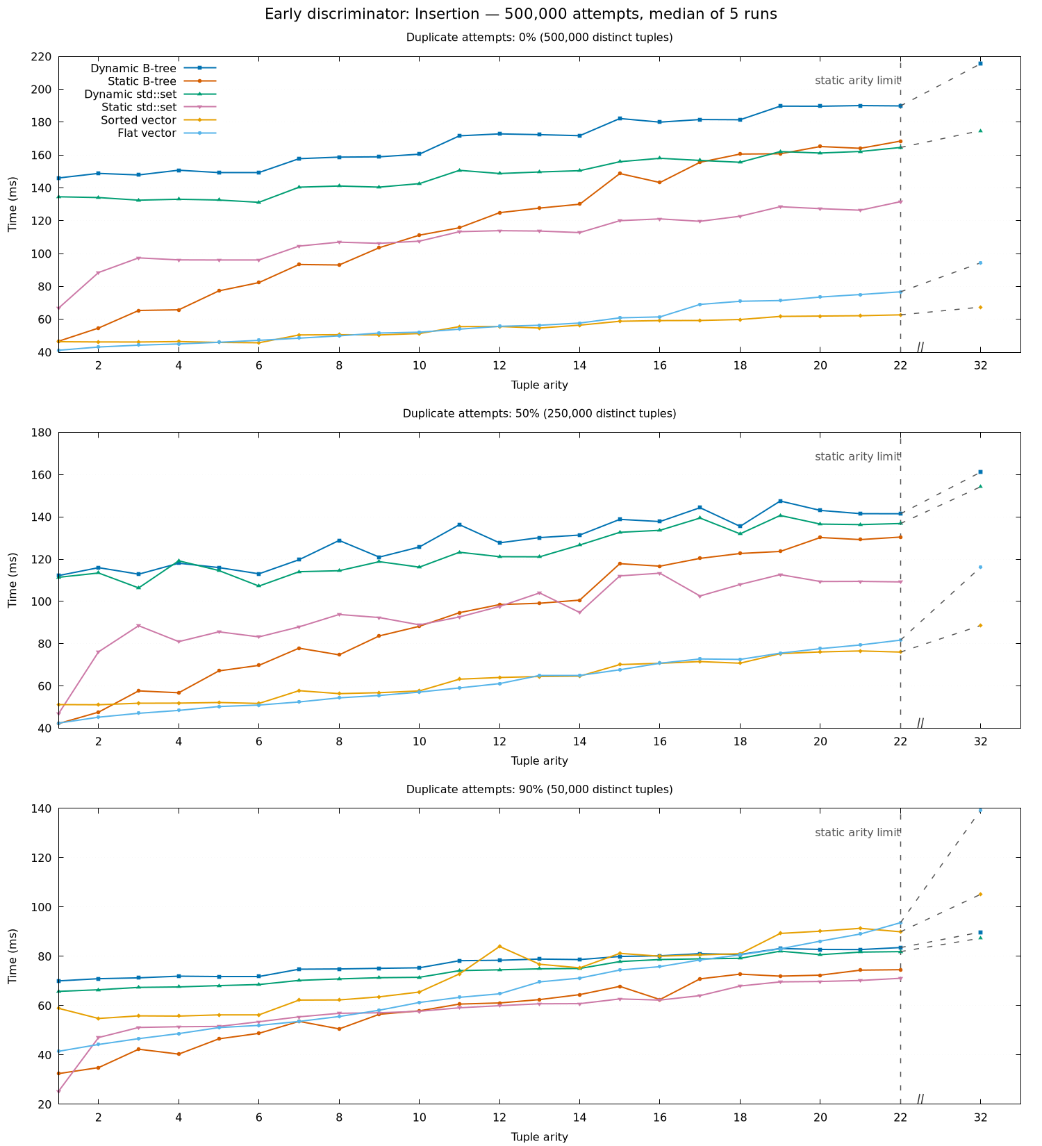
The position of the first differing column has a substantial effect on build time. At arity 22 with no duplicates, dynamic B-tree insertion took 190 ms with the early discriminator and 313 ms with the late discriminator. Flat-vector construction took 77 ms and 186 ms respectively. In the late profile, distinct tuples share the first 21 columns, so lexicographic comparisons must inspect the final column.
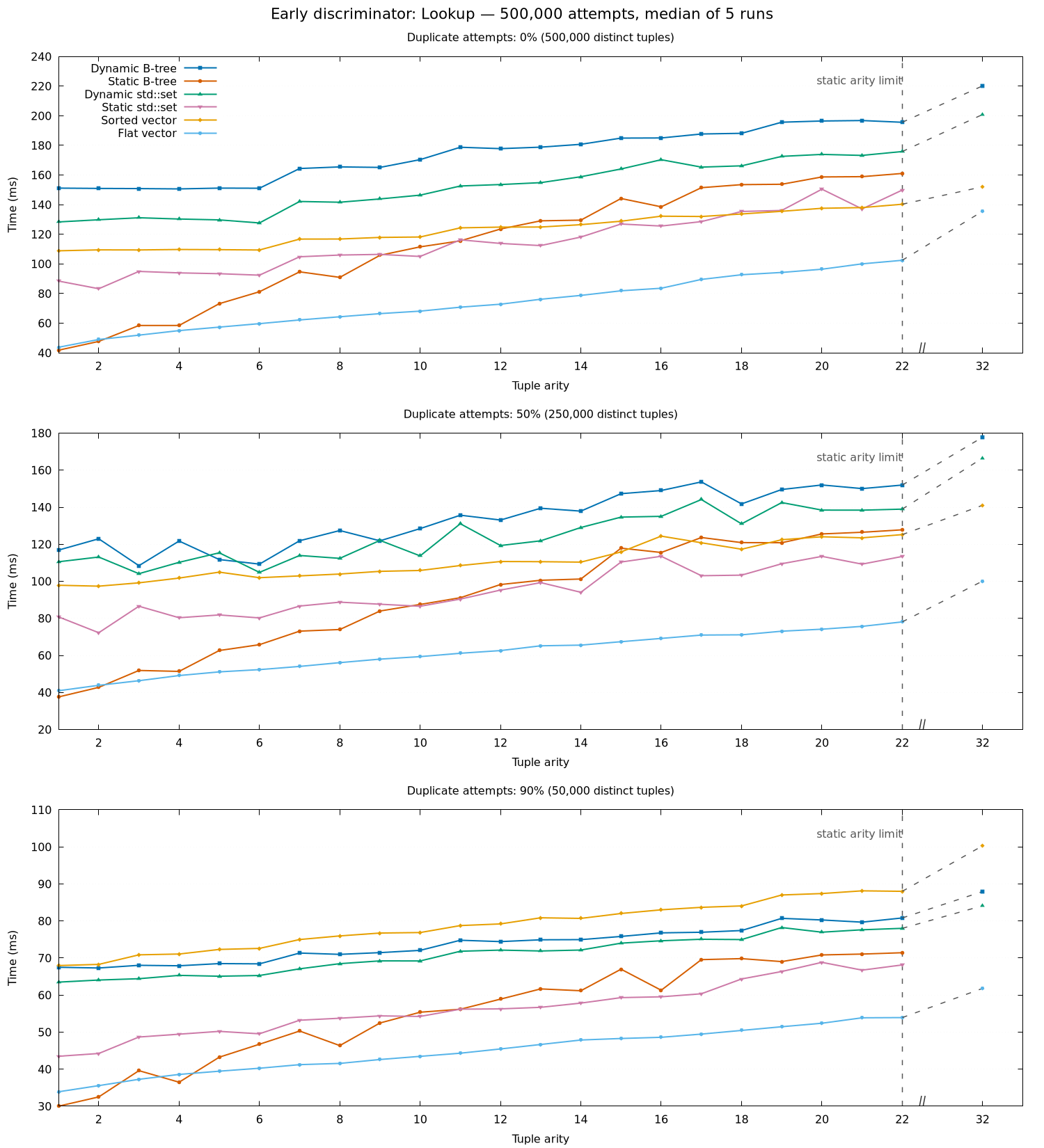
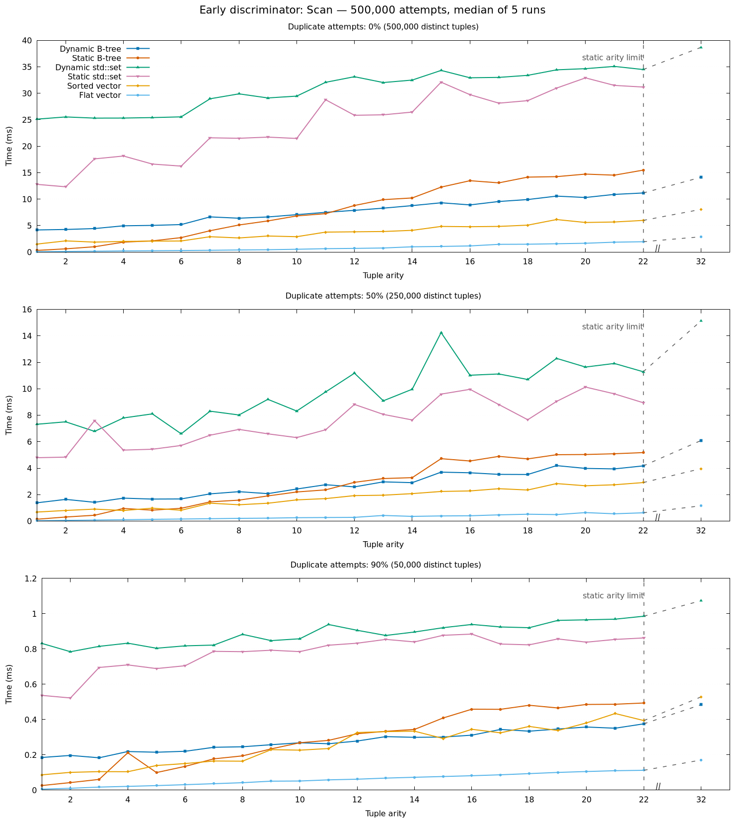
The table counts which strategy had the lowest median time across the measured arities. Static strategies cover arities 1–22; dynamic strategies also include arity 32. Counts are per operation and duplicate rate, so they describe how often each strategy led rather than the size of its lead.
| Comparison profile | Duplicate attempts | Fastest insertion | Fastest lookup | Fastest scan |
|---|---|---|---|---|
| Early | 0% | Sorted vector: 16/23; flat vector: 7/23 | Flat vector: 21/23; static B-tree: 2/23 | Flat vector: 23/23 |
| Early | 50% | Flat vector: 12/23; sorted vector: 10/23; static B-tree: 1/23 | Flat vector: 21/23; static B-tree: 2/23 | Flat vector: 23/23 |
| Early | 90% | Static std::set: 14/22; static B-tree: 7/22; flat vector: 1 at arity 7; dynamic std::set: 1 at arity 32 |
Flat vector: 20/23; static B-tree: 3/23 | Flat vector: 23/23 |
| Late | 0% | Flat vector: 22/23; sorted vector: 1/23 | Flat vector: 22/23; static B-tree: 1/23 | Flat vector: 23/23 |
| Late | 50% | Flat vector: 17/23; static std::set: 4/23; static B-tree: 2/23 |
Flat vector: 22/23; static B-tree: 1/23 | Flat vector: 23/23 |
| Late | 90% | Static std::set: 15/22; static B-tree: 7/22; dynamic std::set: 1/23 at arity 32 |
Flat vector: 21/23; static B-tree: 2/23 | Flat vector: 23/23 |
Charts
Each chart shows one operation across the three duplicate rates. The broken x-axis places arity 32 after arity 22; dashed guides connect the dynamic strategies’ measured endpoints across the unmeasured range.
Early discriminator
Late discriminator
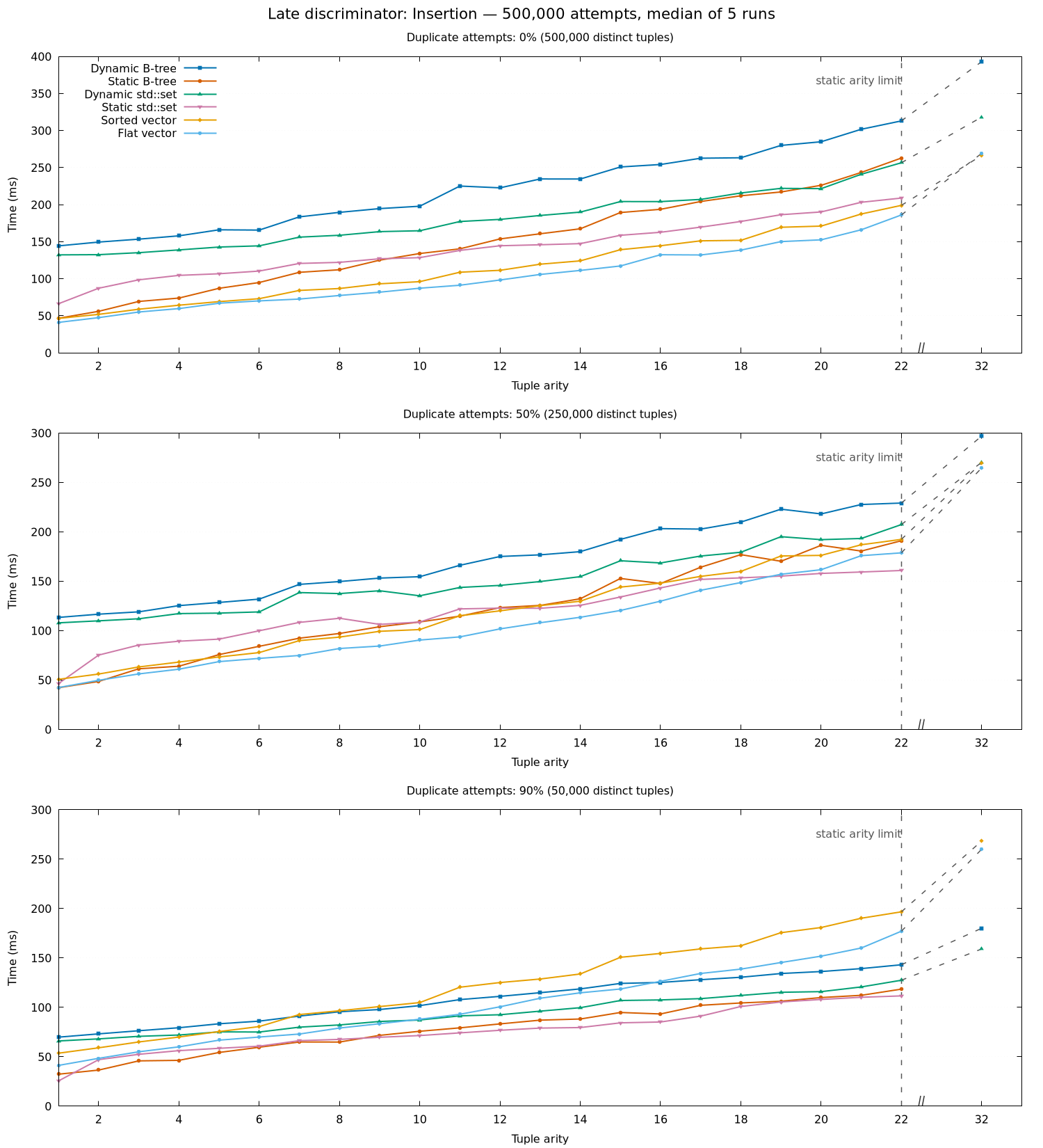
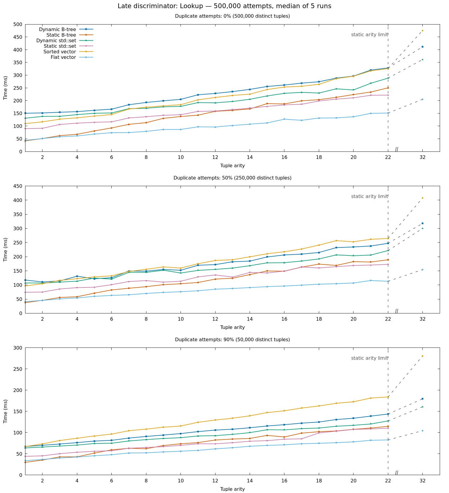
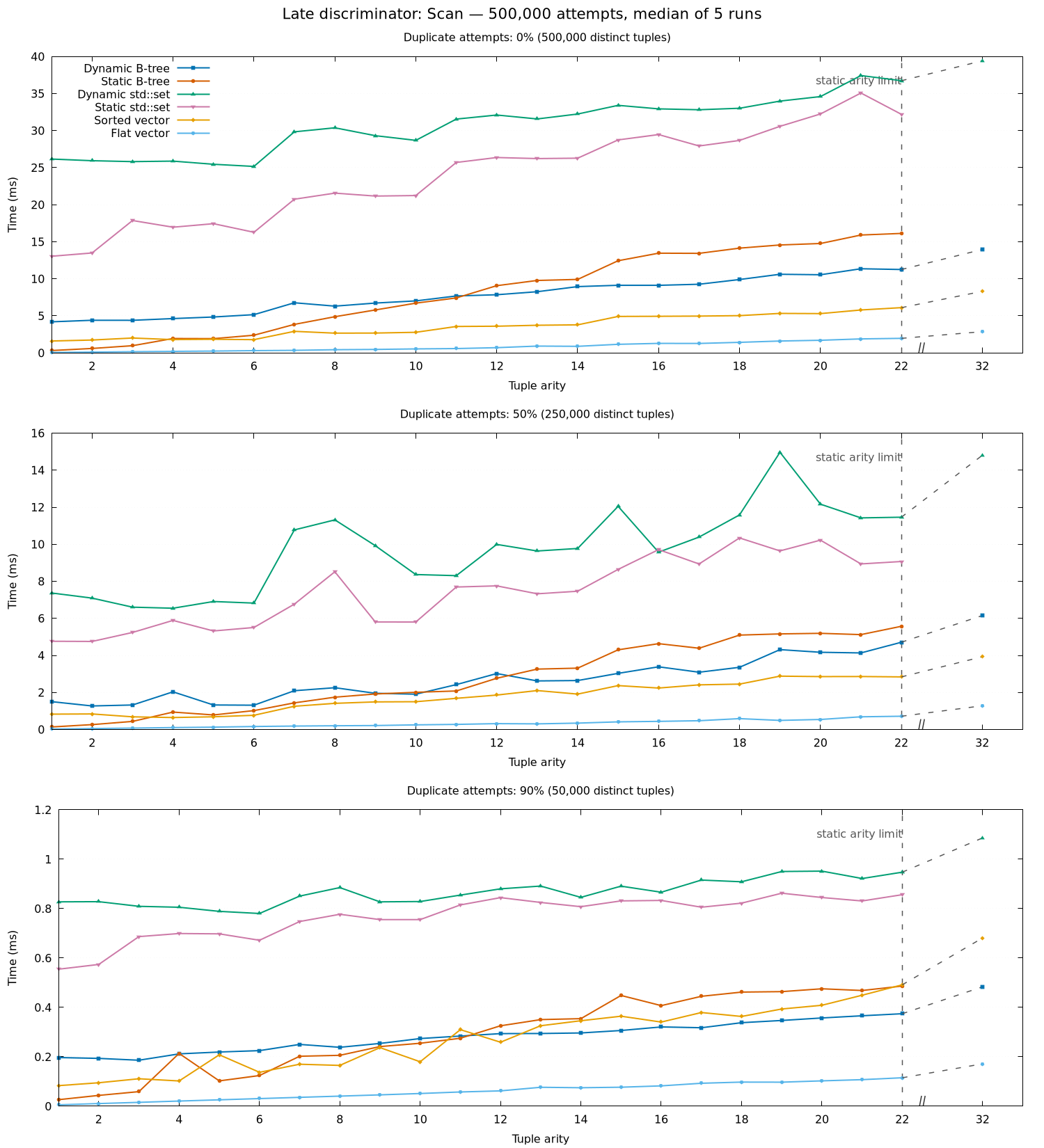
Across arities, flat-vector lookup took 0.44–0.58 times the sorted-vector lookup time, depending on profile and duplicate rate. Flat-vector scans took 0.17–0.23 times the sorted-vector scan time. Flat-vector insertion often led when duplicates were uncommon. At 90% duplicates, static std::set or the static B-tree led most arities because they reject duplicates during insertion, while vector strategies still sort the full batch.
These results motivate a phase-based design to test in the interpreter: use an incrementally updated structure while a relation may grow, then consider a contiguous read-only representation once it is complete and likely to be scanned often. The benchmark does not measure this transition. It builds each candidate from the same batch input and excludes the cost of converting a live B-tree to a vector. Whether conversion pays off also depends on how many lookups and scans follow, and on the query patterns.
Limits and next experiments
These are synthetic results from one machine, not a prediction for every Datalog program. Every lookup is a successful full-tuple lookup; the benchmark does not include misses, prefix or index searches, range queries, joins, concurrent readers, or memory measurements. The two profiles deliberately represent early and late lexicographic differences, while real relations can have mixed prefix distributions.
An exact hash-based deduplication stage is a plausible next comparison: use a hash table with full tuple equality to retain only unique tuples, then sort those unique tuples into the flat vector. A Bloom filter alone cannot safely discard a possible duplicate because false positives could drop valid tuples. No hash-based or Bloom-filter strategy is included in the current CSV.
Reproduce the benchmark
The benchmark source code is available on GitHub.
Configure and build the explicitly excluded benchmark target from the repository root. For general CMake options and dependencies, see the Soufflé build guide.
cmake -S . -B build/dynamic-btree-benchmark
cmake --build build/dynamic-btree-benchmark \
  --target dynamic_btree_benchmark -j12
Run it with the number of insertion attempts. The argument is optional; the default is 25,000. This command writes the same 500k-attempt CSV used in this article:
mkdir -p benchmark-results
build/dynamic-btree-benchmark/src/tests/dynamic_btree_benchmark \
  500000 > benchmark-results/dynamic-btree-duplicates-500k.csv
The executable prints CSV to standard output. Its matrix has both comparison profiles, duplicate rates of 0%, 50%, and 90%, arities 1–22 and 32, and five timing repetitions per implementation and case. The CSV includes a comparison_profile column and has 816 result rows for the 500k run.
To regenerate the six charts from any benchmark CSV, install Python 3 and gnuplot, then run:
python3 benchmark-results/plot_dynamic_btree_benchmark.py \
  benchmark-results/dynamic-btree-duplicates-500k.csv
Charts are written beside the CSV by default. Pass --output-dir PATH to choose another directory.
Results data
Download the raw benchmark CSV (816 result rows).